INL1: India built environment decarbonisation
India’s built environment is experiencing rapid growth driven by urbanisation, but its energy use intensity is high: commercial buildings average 100+ kWh/m²/year compared to 30–70 kWh/m²/year for vernacular buildings. 80% of India’s energy demand is met by coal, oil and solid biomass.
The essay argued that decarbonisation requires action across five areas: strengthening and enforcing the Energy Conservation Building Code (ECBC 2017) and National Building Code (NBC 2016); expanding LEED and GRIHA green building certification; integrating lessons from vernacular architecture (passive cooling, thermal mass, cross-ventilation, natural daylighting); scaling rooftop solar and grid modernisation for rural electrification; and reorienting investment towards retrofitting existing stock rather than only new construction.
Three Indian case studies were analysed: the Infosys Mysore campus (LEED Platinum — 40% more energy-efficient than ASHRAE baseline, 58% water saving, 90% daylit floor area, 10% recycled construction material); the Delhi Metro (carbon-neutral since transitioning to green standards under CDM/Gold Standard, with ~14 million sq ft of Phase-III construction certified to IGBC Green); and the Smart Cities Mission (98–110 cities competing to implement circular-economy and smart-grid principles linked to SDG 11).
The vernacular architecture section analysed Kerala’s Nalukettu typology (central open courtyard, laterite walls, terracotta tiled roof on wooden beams, four-hall layout) as a climate-responsive design model for tropical monsoon conditions, and Rajasthan’s stepwells and havelis as passive cooling precedents for arid climates. The key transferable principles were: orientation along prevailing winds, thermal mass, high ceilings, cross-ventilation, and minimised reliance on mechanical cooling.
INL2: IDA ICE parametric simulation
The baseline condition was established by adjusting maximum heating and cooling power in IDA ICE to achieve a Predicted Percentage of Dissatisfied (PPD) value of approximately 6%. Maximum power settings were then fixed and individual parameters varied to isolate their effect on AHU power, district heating peak demand and total delivered energy.
Heat exchanger addition (effectiveness = 0.7)
AHU power: 38.6 → 8.6 kW78% reduction in air-handling power
DH peak: 63.1 → 32.8 kW48% reduction in district heating peak
Total energy: 160,733 → 118,890 kWh26% reduction in delivered energy
Heat exchanger addition was the most impactful single change tested. Recovering heat from exhaust air at 70% effectiveness reduced the ventilation heating load substantially, cutting both AHU power demand and the district heating peak nearly in half.
Other parametric changes
- External window blinds: No significant change to any energy metric. External shading had negligible effect in the baseline Stockholm climate scenario.
- Building orientation (E–W → N–S): Slight increase across all values. The baseline E–W orientation is marginally better for this climate and geometry.
- Location change to Barcelona: Eliminated heating demand entirely (PPD below 15% without any heating power). Cooling requirement: 40 kW ground floor, 50 kW upper floor. A new baseline calibration was required since the mild Mediterranean climate makes the Stockholm heating system parameters irrelevant.
INL3: Supply system comparison — 11 configurations
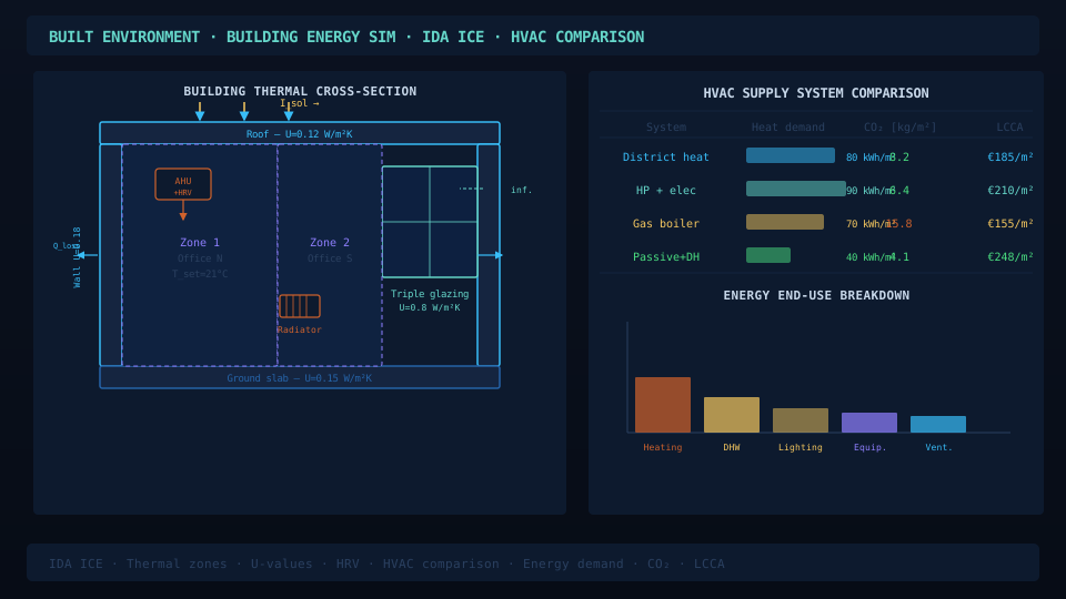
The reference system uses an oil boiler for heating and a liquid chiller for cooling. Ten alternative configurations were simulated, all evaluated on annual bought energy, primary energy used and CO&sub2; emissions:
Reference (oil boiler): 111,963 kWh bought217,524 kWh primary — 41,232 kg CO&sub2;
GSHP + liquid chiller: 80,407 kWh bought196,806 kWh primary — 33,063 kg CO&sub2; (−28%)
GSHP + full PV: −25,819 kWh boughtNet export to grid — negative CO&sub2; balance
Key findings from the 11-configuration sweep:
- Turbo vs reciprocating compressor (chiller): Switching to a turbo compressor increased bought energy and emissions for both 40 kW and 50 kW cooling capacities, indicating the reciprocating compressor is more efficient in this application. Higher cooling capacity also increased all metrics.
- District heating and cooling: Counter-intuitively, switching to district H&C produced the worst result of all configurations — bought energy rose to 148,461 kWh and CO&sub2; to 47,139 kg. This is likely due to the district system’s primary energy conversion factor in the modelled scenario.
- GSHP + liquid chiller: Reduced bought energy by 28% and CO&sub2; by 20% versus the oil boiler reference, confirming the higher efficiency of ground-source heat extraction over combustion heating.
- GSHP with adjusted top-up/rated split (20 kW top-up, 10 kW rated): Further improved primary energy (187,574 kWh) and CO&sub2; (31,512 kg) relative to the standard GSHP configuration, showing that auxiliary heater sizing affects overall system efficiency.
- GSHP + full-area PV panels: Net negative bought energy (−25,819 kWh) and negative CO&sub2; (−11,436 kg) — the building becomes a net energy exporter. With half the PV area, the system returns to positive bought energy (27,287 kWh), confirming the size threshold between self-sufficiency and export.
- ASHP + liquid chiller: Better than the oil boiler reference (83,132 kWh bought, 33,653 kg CO&sub2;) but consistently worse than GSHP configurations across all metrics, due to the lower COP of air-source vs. ground-source heat extraction.
Summary ranking (bought energy, annual)
- 1st: GSHP + full PV — −25,819 kWh (net export)
- 2nd: GSHP + turbo chiller 40 kW — 79,814 kWh
- 3rd: GSHP + liquid chiller — 80,407 kWh
- 4th: GSHP + top-up adjusted — 87,717 kWh
- 5th: ASHP + liquid chiller — 83,132 kWh
- Last: District H&C — 148,461 kWh
Limitations
- INL2 simulations are parametric — one variable changed at a time from a fixed baseline; combined effects (e.g. heat exchanger + PV) were not explored in INL2.
- INL3 used pre-configured .idm system files; the screw compressor configuration produced a simulation error and could not be evaluated.
- Primary energy and CO&sub2; conversion factors are embedded in the IDA ICE system files and may not reflect real-time grid carbon intensity or future decarbonised grid scenarios.
- The Barcelona location change in INL2 required a new PPD-based baseline and is not directly comparable to the Stockholm baseline results.