Day-Ahead Heating Demand Forecasting for a University Building

The problem

Accurate day-ahead heating demand forecasts allow building operators and district heating networks to optimise production scheduling, reduce peak-load costs and improve integration of variable renewable supply. Physics-based building models are computationally expensive and require detailed building geometry and materials data; data-driven models offer a faster, more scalable alternative when metered data is available.

The goal was to compare three models of increasing architectural complexity on the same dataset and determine whether the additional compute cost of deeper networks is justified by the accuracy gain — a practically important question for energy management systems that need to run forecasts continuously.

Dataset and feature engineering

The dataset comprised one year of hourly measurements from the KTH U-Building sensor network. Analysis was restricted to the heating season (1 October – 30 April) to avoid injecting summer cooling behaviour that would add noise without improving heating predictions.

Eight input features were used, combining direct sensor readings with three engineered temporal variables:

• Sensor readings: outdoor temperature, global radiation, wind speed, wind direction, relative humidity
• Engineered: Hour of day (0–23) — captures occupancy-driven demand patterns (higher during building-use hours)
• Engineered: Chronological day (1–365) — captures seasonal variation in heating load
• Engineered: Weekday (1–7) — distinguishes weekday/weekend occupancy patterns typical of educational buildings
• Output: Space heating demand (kW)

Variables closely correlated with the output — volumetric cooling flow, cooling demand — were intentionally excluded to avoid data leakage and to keep the model generalisable to buildings without those sub-meters.

Data cleaning pipeline

The raw dataset had 5,112 hourly rows. Cleaning proceeded in two stages:

• Initial cleaning: Wind direction values outside 0–360° removed (10 rows); negative space heating demand removed (2 rows); duplicate timestamps resolved by substituting nearest-neighbour values. Remaining: 5,100 rows.
• Mahalanobis outlier removal: Multivariate outliers identified using Mahalanobis distance (threshold 3.5σ), which accounts for cross-variable correlation structure rather than single-variable extremes. This removed 106 additional rows (51 global radiation, 30 space heating, 16 wind speed, 9 outdoor temperature). Final dataset: 4,992 rows.

After cleaning, wind speed maximum dropped from 3,276.7 to 14.5 (units consistent with sensor range), and space heating minimum went from −155.92 kW to 1.26 kW, confirming the outlier removal was well-targeted. MinMaxScaler (scikit-learn) normalised all features to [0, 1] before model training.

Model architectures and hyperparameter search

All three models share the same forward-propagation / backpropagation / gradient-descent framework. The hyperparameter search space was identical across all models:

• Learning rate: 0.1–1.0 in steps of 0.1
• Iterations: 1,000 / 2,000 / 3,000
• Nodes per hidden layer (SNN/DNN): 1–10
• Number of hidden layers (DNN only): 2–10

Two simplifying assumptions were applied to contain the search space: ReLU activation for all hidden layers (no activation-function tuning), and equal node count across all hidden layers in the DNN. The output layer used sigmoid in all models.

Optimal architectures found by trial and error:

• Logistic regression: no hidden layers (baseline)
• SNN: 1 hidden layer, 4 neurons
• DNN: 6 hidden layers, 8 neurons each

Results

The accuracy gap between SNN and DNN on the test set is only 0.33 percentage points, while the DNN takes 10× longer to train (7 s vs 0.69 s). Logistic regression trains in under 0.1 ms. From an energy management deployment perspective — where the model may run continuously or retrain daily — this runtime ratio strongly favours the SNN.

Runtime and efficiency trade-off

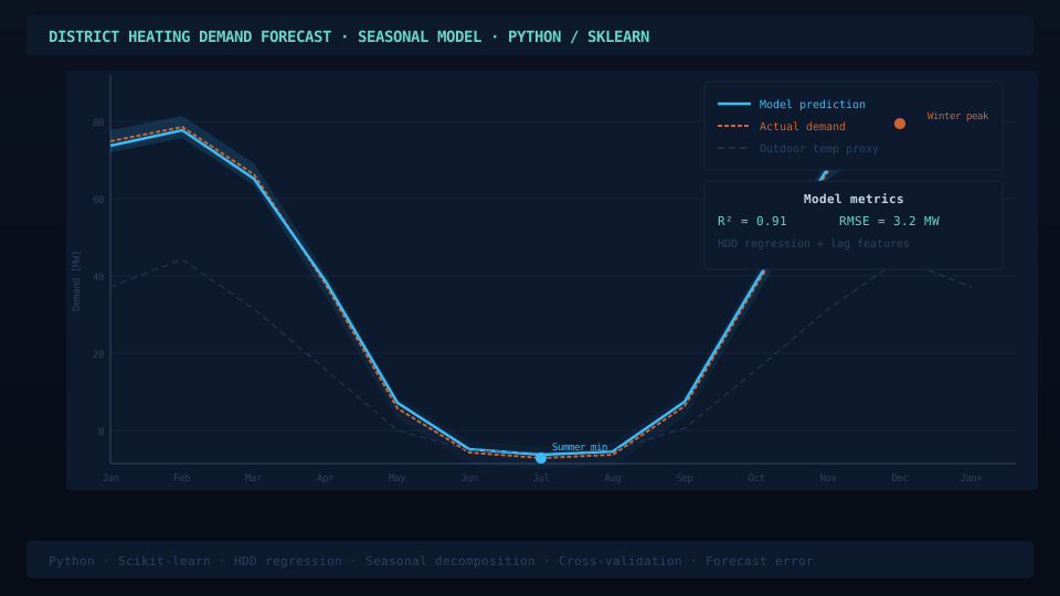
The DNN’s 2.2-percentage-point drop from test accuracy (93.72%) to validation accuracy (91.53%) on the January 12 validation day indicates the DNN has partially memorised the training distribution. The SNN’s test–validation gap is only 1.02 pp, confirming better generalisation. The conclusion is that SNN is the operationally preferred architecture for this task at this dataset scale.

Peak value limitation

All three models underpredict at extreme heating demand peaks. MAE as an optimisation metric weights all errors equally; large errors at rare peak-demand hours are outvoted by the large number of well-predicted mid-range hours. Two approaches were identified to address this:

• Switch the optimisation metric to R², which penalises failure to explain variance and would drive the model to fit peaks better
• Increase training data volume or temporal resolution to give the model more examples of high-demand conditions

Limitations

• Activation function fixed to ReLU; other functions (tanh, Leaky ReLU) were not evaluated and could affect convergence behaviour.
• DNN constrained to equal node count per layer — tapered or pyramidal architectures were not explored.
• Model trained on a single building; generalisation to other building types or climates requires retraining on new data.
• Summer months excluded; a year-round model would need a cooling-season counterpart or a single multi-season model.
• Correlation analysis to formally rank feature importance was not performed; solar irradiation and outdoor temperature are expected to be dominant predictors based on the literature, but this was not verified quantitatively in the study.