HA1 — Q1: Floating-point precision and catastrophic cancellation
Two expressions D = (a+b)+c and E = a+(b+c) were evaluated in single (float32) and double (float64) precision for two test cases involving large nearly-equal operands, to demonstrate loss of associativity and catastrophic cancellation.
- Machine epsilon: float32 = 1.19×10³; float64 = 2.22×10³
- Smaller case (a−b≈1): Single precision E = 1.0 (D = 1.333) → 25% error. Double precision E ≈ 1.333334100 → error 3.7×10³%.
- Larger case (a−b≈1, magnitudes ∼10³): Single precision E = 0.0 (D = 0.333) → 100% error (complete cancellation). Double precision E = 1.375 (D = 1.333) → 3.1% error.
Errors far exceed machine epsilon in both cases, confirming that the source is catastrophic cancellation from subtraction of nearly-equal large numbers, not isolated rounding. Even double precision suffers significant error when magnitude differences are extreme.
HA1 — Q2: Numerical differentiation of cos(x) at x = 0.2
Forward difference (O(Δx) truncation) and central difference (O(Δx²) truncation) were compared against the analytical derivative −sin(0.2) across Δx from 10³ to 0.1.
At large Δx, truncation error dominates (slopes consistent with O(Δx) and O(Δx²) on log–log plots). At very small Δx, round-off error from subtracting nearly-equal numbers dominates, causing errors to rise again. The minimum error is found at the crossover. Central differencing achieves lower minimum error because its O(Δx²) truncation term allows a larger optimal Δx where round-off is smaller.
HA1 — Q3: 2D steady-state heat conduction (Laplace equation)
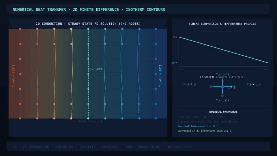
The 2D Laplace equation was solved on a steel plate (L = 8 cm, M = 4 cm) with fixed boundary temperatures using finite-difference discretisation, comparing 5-point (second-order) and 9-point (fourth-order) stencils at multiple grid resolutions.
A 9×9 coefficient matrix was constructed for the small plate (L = 8 cm, M = 4 cm, Δx = 2 cm, Δy = 1 cm). For the large plate, temperatures at three representative interior points were evaluated:
- Coarsest (Δx = Δy = 2 cm, 5-pt): T(16,6) = 393.527 K, max error 0.721 K
- Fine grid (Δx = Δy = 1 cm, 5-pt): max error 0.187 K — 74% reduction
- Fine grid (Δx = Δy = 1 cm, 9-pt): max error 0.055 K
- Most accurate (Δx = 1 cm, Δy = 0.5 cm, 9-pt): max error 0.038 K
Practical conclusion (per professor guidance): the 5-point scheme at Δx = Δy = 1 cm (error < 0.2 K) provides very good accuracy at significantly lower computational cost than the 9-point scheme. Δx = 2 cm gives acceptable quick estimates; higher-order schemes are valuable for verification but not always necessary in engineering practice.
HA2 — Q1: Time-stepping to steady state (Euler vs RK4)
The HA1 Q3 plate problem was revisited using explicit time-marching instead of direct linear system solution, with Δx = Δy = 1 cm and a 5-point stencil. Convergence criterion: maximum residual |R| < 10³.
Stability analysis (2D Fourier stability for explicit diffusion): Δtmax = Δx² / (4α).
At |R| < 10³, both schemes agree with the direct HA1 solution to within 0.01 K. At |R| < 10³ the difference grows to ~0.1 K. RK4’s larger permissible step size and faster convergence make it the more efficient time-marching scheme for this problem, even accounting for its 4 function evaluations per step.
HA2 — Q2: 1D advection — Lax–Friedrichs vs Lax–Wendroff
The linear advection equation ∂u/∂t + U∂u/∂x = 0 was solved on L = 20 m with U = 4 m/s, 100 grid points, sinusoidal initial condition, and Courant number C = 0.5 (well within the stability limit of 1). Solutions were advanced to t = 1, 2, 3 s.
- Lax–Friedrichs (LF): 2nd-order space, 1st-order time. Strongly dissipative — wave amplitude significantly reduced by t = 3 s. L1 error consistently higher at all times.
- Lax–Wendroff (LW): 2nd-order in both space and time. Amplitude and phase preserved throughout. L1 error substantially lower than LF at all times evaluated.
LF’s numerical diffusion arises from its first-order time treatment adding an artificial viscosity term proportional to (Δx)²/Δt. LW eliminates this term at second order. Practical guidance: LF remains useful for robustness with discontinuities or shock-capturing; LW is the correct choice for smooth wave propagation.